In my article about creating a script to help process my family finances, I mentioned a spreadsheet function called SUMPRODUCT. Let me explain a little more clearly how it works.
The SUMPRODUCT function is available in LibreOffice Calc and Microsoft Excel, as well as other programs like Google Sheets. As the name suggests, it returns the sum of the products between the arrays in the arguments.
Examples of SUMPRODUCT in Action
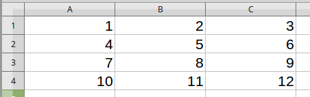
Here's an example. Take the following table of values:
and the following formula:
=SUMPRODUCT( B1:B4, C1:C4 )
This is the equivalent of:
\(B1 \times C1 + B2 \times C2 + B3 \times C3 + B4 \times C4\)
or
\(1 \times 2 + 3 \times 4 + 5 \times 6 + 7 \times 8\)
which is 100.
This also works for arrays of more than a single column (or row):
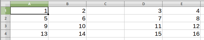
=SUMPRODUCT( A1:B4, D1:E4 )
is
\(1 \times 3 + 2 \times 4 +5 \times 7 + 6 \times 8 +9 \times 11 + 10 \times 12 +13 \times 15 + 14 \times 16\)
which is 732.
And this works for multiple arrays as well, holding that each array has the same dimensions as all the others.
=SUMPRODUCT( A1:A4, B1:B4, C1:C4 )
Gives
\(1 \times 2 \times 3 + 4 \times 5 \times 6 + 7 \times 8 \times 9 + 10 \times 11 \times 12\)
which is 1950.
All this can be done with simpler formulae and intermediate data fields; but then again, all this can be done by hand on paper, or by a dozen carefully trained monkeys with sticks and stones. A cost-benefit analysis may be in order.
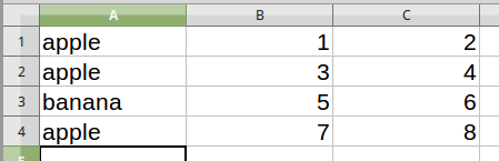
What's interesting about SUMPRODUCT, and what makes it useful for my situation, is the ability to apply conditions on the arrays. Suppose we have the following table, and we want to filter the results:
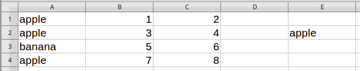
If you only want the sum of the products for all the apples, you can use this formula:
=SUMPRODUCT( A1:A4 = E2, B1:B4, C1:C4 )
What that first argument, A1:A4 = E2, does is inspect each value in the array A1:A4 and checks if it's equal to the value in E2 (it also works if you put in "apple" directly into the formula). This turns it into a boolean array, containing only true or false. In some spreadsheet programs, you have to convert the trues and falses into numbers, but in LibreOffice, it will automatically coerce true into 1 and false into 0 whenever the situation requires it.
The formula is then equivalent to:
\(1 \times 1 \times 2 + 1 \times 3 \times 4 + 0 \times 5 \times 6 + 1 \times 7 \times 8\)
which is 70.
The falses become zeroes, which when multiplied by any value becomes zero, and cancels out that term. This also works with other mathematical checks, like < or >.
How I Used It
So here's how I used it. I have a table that looks like this (somewhat simplified):
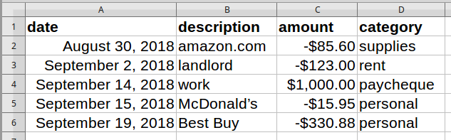
Suppose I want to know my total expenditures for the month of September. My source data is in column A, and I can select the entire column using A:A. Unfortunately, I can't type in A:A = "September" as I did earlier, since the date is not equal to the name of a particular month. However, there is another function called MONTH that returns a number from 1 to 12 for what month a particular date represents, so I can write, MONTH(A:A) = 9. If the target date is, for example, in cell E2, then I can also write, MONTH(A:A) = MONTH(E2).
The data may contain entries from more than one year, and we don't want data from last September in the results, so we also have to add YEAR(A:A) = YEAR(E2) to make sure both the month and the year are the same. Here, we don't care about the date within the month.
Since in this example we want expenditures only, we add a condition that the values (in column C) must be less than zero: C:C < 0.
Lastly, we can't forget the data in column C itself: C:C. Don't forget that the previous array, C:C < 0 only gives us ones for when the value is less than zero, and zeroes for when the value is greater than or equal to zero.
Put it all together, and you get: =SUMPRODUCT( MONTH(A:A) = MONTH(E2), YEAR(A:A) = YEAR(E2), C:C < 0, C:C ).
It looks like a lot - and it kinda is - but it's really quite simple, and it fits in one formula in one cell.
To report all the incomes of a particular month, simply replace C:C < 0 with C:C > 0. To report the net total of the month, just remove that argument altogether.
As a final example, I want a table of totals grouped by category like this:
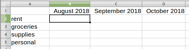
If the data (from the previous table) is on another sheet called Data, then we can access values using the name of the sheet, then a dot, then the address of the cell or cells like normal (eg: Data.A1, Data.B5:C7, Data.A:A, etc). The formula here on the Totals sheet in C2 would then be:
=SUMPRODUCT( MONTH(Data.A:A) = MONTH(C1), YEAR(Data.A:A) = YEAR(C1), Data.D:D = A2, Data.C:C )
This compares the month and year of the data in column A from the Data sheet with the month and year of the target date in cell C1 of the Totals sheet, filters out the categories that don't match the text in A2, then adds up the amounts in column C of the Data sheet.
To make things a little easier to use, we can use the dollar sign to lock the row, the column, or both. That way, when we "fill" down and across, the formulas will change according to the target month and category.
=SUMPRODUCT( MONTH(Data.$A:$A) = MONTH(C$1), YEAR(Data.$A:$A) = YEAR(C$1), Data.$D:$D = $A2, Data.$C:$C )
When filled down, only the 2 in Data.$D:$D = $A2 will change (matching the category), and when filled right, only the C in the first two arguments will change (matching the month).
Is It Better?
There are a couple of benefits from using SUMPRODUCT in this situation instead of something else. For one, it's much more neat and tidy than having a whole bunch of extra columns (or separate sheets) for intermediate calculations. Second, because the date and category of each transaction is not very predictable, it's nice to have a formula which can check the entire column of data and automatically filter for the appropriate entries. It's also nice to be able to simply "fill" the cells down all my categories, then across for each new month, rather than target each month by hand.
The main drawback here is that it's slow. Because I'm checking down the entire lengths of the columns, the "Totals" sheet consumes a lot of processing power. Most of the comparison calculations are duplicated work. I'm not sure what shortcuts the program makes, but LibreOffice on my laptop sometimes takes up to thirty seconds to load the sheet.
As I've mentioned before, speed is not a high priority when analyzing my finances. Also, I'm only ever using this document a couple times per month. Nevertheless, I'm sure there are optimizations that I can make without sacrificing convenience. Unfortunately, spreadsheets are not my area of expertise. Maybe I should consult those trained monkeys. If you have a suggestion, please let me know.